Low-Cost Shaft Eccentricity Monitoring
A stray-flux magnetometer rig that measures shaft eccentricity to 10.6 % mean error and tells static from dynamic without a miss — for £148.55, against £1,500–2,000 of eddy-current probes.
Evidence
- 10.6 %Magnitude errormean absolute, target 15 %
- 80.9 µmExpanded uncertaintyk = 2, GUM
- 30/30Classificationboth classifiers
- £148.55Instrumentationvs £1,500–2,000
- 498 HzAngle-synchronous rate
- 20.0 µmBaseline runout± 1.0, target ≤ 25
Case study
The problem
- Eddy-current probes resolve shaft eccentricity properly and cost £1,500–2,000 for the dual-channel set — an order of magnitude past a teaching lab’s budget.
- Hall-effect magnetometers cost about a hundredth of that and are worse in every respect that matters: non-linear, noisier, geometry-dependent. The question is where they are nonetheless good enough.
The design
- Two orthogonal MLX90393 magnetometers reading the stray field off a 6 mm diametrically magnetised target on the shaft; an AS5600 encoder angle-stamps every sample at 498 Hz on an ESP32-S3.
- Static eccentricity comes from printed collars with the bore offset 0.25–1.00 mm; dynamic eccentricity from clamp-on masses at a fixed radius. Every fixture was micrometre-verified and the verified value — not the nominal — is the ground truth.
- Angle-synchronous averaging over 20 revolutions, then three features: RMS orbit radius, the 2×/1× harmonic ratio R, and the inter-channel phase difference.
What I did
- Designed and built the whole instrument — rig, fixtures, firmware, processing pipeline.
- Wrote a GUM uncertainty budget rather than quoting a scatter band. That is what showed the calibration-fit residual to be three times the next largest term.
- Benchmarked a transparent two-feature rule against a Random Forest, and argued for the rule.
How it was tested
- Thirty acquisitions: ten conditions, three independent repeats, at 1000, 1500 and 2000 RPM.
- Baseline shaft runout measured at 20.0 ± 1.0 µm before any fixture went on — twelve times smaller than the smallest eccentricity tested, which is what makes the rest of the numbers mean anything.
- Magnitude scored against the micrometre-verified offsets, not against the values the collars were meant to be.
Result
- 10.6 % mean absolute magnitude error across the static cases, inside the 15 % target. Expanded uncertainty 80.9 µm at k = 2.
- Both classifiers separated healthy, static and dynamic on all 30 repeats. The rule shipped.
- Validated envelope stated as an envelope — 1000–2000 RPM, 0.23–0.96 mm. Above it, rig dynamics contaminate the 2× harmonic, and the report says so.
The hardware
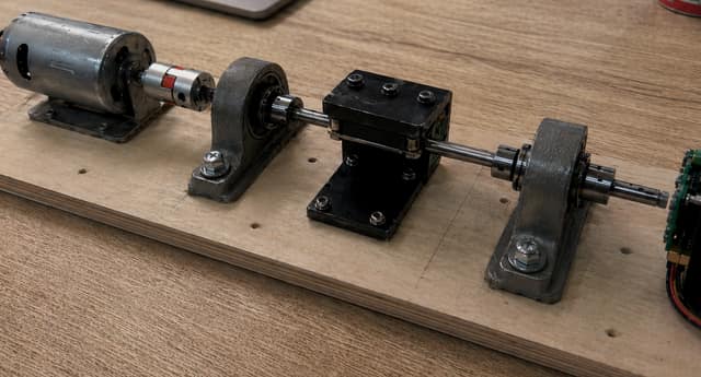
The rig as built. Motor, jaw coupling, two pillow blocks 182 mm apart on an 8 mm ground shaft; the sensor tower straddles the shaft at mid-span and the encoder reads the free end. Baseline runout on this assembly was 20.0 ± 1.0 µm.

Static and dynamic eccentricity leave different signatures in the shaft orbit, which is what makes the fault worth monitoring. The instrument that resolves them properly is a dual-channel eddy-current probe set, and at £1,500–2,000 an installation it prices teaching labs out of continuous monitoring entirely.
Two Hall-effect magnetometers cost about a hundredth of that and are considerably worse: non-linear, noisier, geometry-dependent. The question is not whether they are as good — they are not — but where the envelope inside which they are good enough actually sits, and what the uncertainty on it is.
Decisions
- 01
Why magnetometers instead of the probes the scoping document specified?
Cost, and the project is about cost. The eddy-current set was quoted at £1,500–2,000, which is an order of magnitude outside the budget the work is arguing for. Two magnetometers at £7.47 a breakout give a 20 µm noise floor — coarser than a probe, but the smallest eccentricity tested was 0.23 mm, and a floor twelve times below your smallest signal is not the thing limiting you.
- 02
Why average by shaft angle rather than by time?
The diagnostic content is angle-locked — 1× and 2× happen once and twice per revolution whatever the speed drifts to. Binning by encoder angle over 20 revolutions suppresses uncorrelated noise by √20 with no assumption that the motor held its speed, which a brushed motor on a PWM driver does not.
- 03
Why publish the rule and not the Random Forest, when both scored 30/30?
Thirty records cannot separate them, so the tie breaks on everything else. The rule is two comparisons against thresholds sitting in visible gaps, needs no training, runs on the microcontroller, and when it is wrong you can see why. The forest answers a question this dataset is too small to ask.
- 04
Why is the one failing case published?
SE02 — the smallest offset at the middle speed — came out at 16.7 % against a 15 % target. It is also exactly what the uncertainty budget predicts: a fixed 81 µm expanded uncertainty is 17.6 % of a 0.23 mm eccentricity. A result that fails where your own error model says it will is evidence the model is right. Deleting it would have been the only dishonest option.